PTQ&QAT方案板端验证注意事项

[颜值即正义]

0 前言

由于部署时数据来源的硬件不同以及应用开发的高效性要求，往往会使得在板端部署阶段的数据准备操作与训练时有所差异。通过阅读本文您可以找到以下问答的答案：

1. 一些常见的图像格式转换以及归一化处理是否支持硬件加速？（请参考本文1.1节）
2. 若部署时数据来源于摄像头，我应该怎么配置？（ptq方案请参考本文1.2.1节，qat方案请参考2.2.1节）
3. 若部署时数据来源于摄像头，可以如何验证板端和PC端模型精度一致性？（ptq方案请参考本文1.2.2节，qat方案请参考2.2.2节）
4. 在什么情况下我需要在预处理时完成量化、数据对齐操作？（ptq方案请参考本文1.2.2&1.3节，qat方案请参考2.2.2&2.3节）
5. 从PTQ方案迁移到QAT方案的话数据预处理方面需要做什么调整？（请参考本文第二章）

1 PTQ方案

PTQ方案：通过地平线提供的hb_mapper工具完成浮点模型向定点模型的转换。该方案只需要用户准备少量的校准数据并配置一份config.yaml文件即可通过一行命令完整模型量化。

1.1 与模型输入信息相关的配置项

yaml配置文件中的输入信息参数组input_parameters决定了在板端部署时需要准备的数据格式，并提供了使用bpu加速数据格式转换和数据归一化操作的配置接口。输入信息参数组的所有配置项如下表所示：

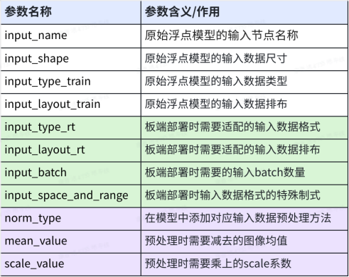
前四个参数为原始浮点模型的输入节点信息，中间四个参数为板端部署时的输入数据格式，通过最后三个参数可以将视觉任务中常用的数据归一化操作配置进模型中使用硬件做加速计算。支持配置的input_type_train和input_type_rt组合以及部署时DNN预测库解析出来的数据格式如下表所示：

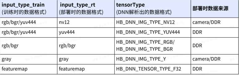
其中nv12支持两种数据分布范围，可通过input_space_and_range参数指定。默认为regular，数值范围为 [0,255]；还可支持 bt601_video，数值范围为[16,235]。

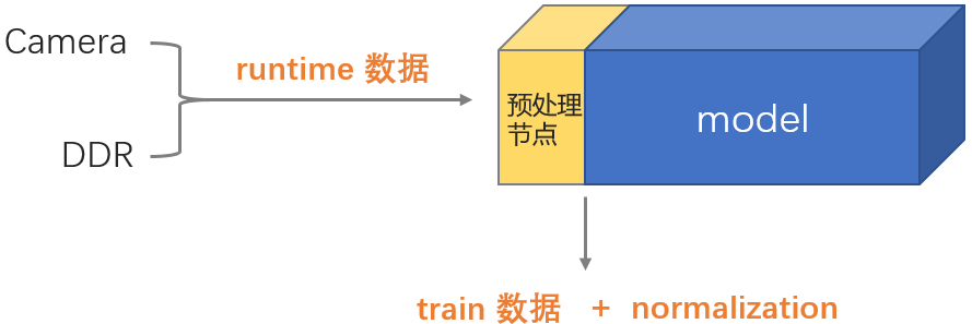
工具通过解析input_type_train、input_type_rt以及norm_type等参数，将为您的模型插入一个预处理节点（该节点为conv节点，耗时非常少），以使用bpu加速数据格式转换和数据归一化操作。如下图所示，在板端进行模型推理时，预处理节点会先将input_type_rt格式的数据转换为input_type_train格式并完成归一化计算，再送入模型进行后续推理。

norm_type参数的配置方式建议参考工具链用户手册norm_type 配置参数说明章节内容。

此外，依据工程部署优化需要，大家可能会使用到编译参数组compiler_parameters中的input_source，配置为resizer的话，则将支持resize操作的硬件加速，具体可参考社区文章resizer模型使用与部署。

1.2 camera输入注意事项

本节我们以yolov5s模型为例，说明camera输入场景下模型转换配置以及模型精度验证的方式和注意事项。yolov5s模型浮点训练时的预处理代码为：

im = cv2.imread(path) 
im = letterbox(im0, self.img_size, stride=self.stride, auto=self.auto)[0]  # padded resize 
im = im.transpose((2, 0, 1))[::-1] # HWC to CHW, BGR to RGB 
im.float() 
im /= 255  # 0 - 255 to 0.0 - 1.0 

1.2.1 模型转换

依据前文1.1节介绍的配置项说明，yolov5s模型的config.yaml文件可按如下配置：

model_parameters: 
  onnx_model: 'YOLOv5s.onnx' 
  march: "bernoulli2" # J5：Bayes 
  output_model_file_prefix: 'yolov5s_672x672_nv12' 
input_parameters: 
  input_type_rt: 'nv12' # 配置nv12时，input_source默认为pyramid 
  input_type_train: 'rgb'  # 训练时的数据格式 
  input_layout_train: 'NCHW' # 训练时的数据排布 
  norm_type: 'data_scale' 
  scale_value: 0.003921568627451 # 1/255 
calibration_parameters: 
  cal_data_dir: './calibration_data_rgb_f32' 
  cal_data_type: 'float32' 
  calibration_type: 'default' 
compiler_parameters: 
  compile_mode: 'latency' 
  debug: False 
  optimize_level: 'O3' 

校准数据预处理代码：

im = cv2.imread(path) 
im = letterbox(im0, self.img_size, stride=self.stride, auto=self.auto)[0]  # padded resize 
im = im.transpose((2, 0, 1))[::-1] 
im.float() 
# im /= 255 该操作已通过yaml文件配置进了模型中 

1.2.2 PC端与板端推理一致性验证

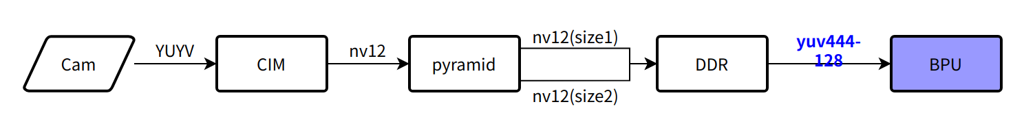
若想验证量化后定点模型的精度，建议可以在PC端验证quantized.onnx模型的精度。由于PC端缺少硬件配合，因此相较于板端需要多做一步操作：将数据处理到input_type_rt的中间类型（nv12对应的中间类型为yuv444_128）。其他数据格式对应的中间类型建议参考工具链用户手册转换内部过程解读相关介绍。

在板端部署时nv12转yuv444_128的操作是在从DDR读取nv12数据时由编译器完成的，如下图所示。在PC端推理quantized.onnx则需自行在预处理时完成该转换。

1. yolov5s_672x672_nv12_quantized.onnx推理示例代码：

import cv2 
import numpy as np 
from PIL import Image 
from horizon_tc_ui import HB_ONNXRuntime 
 
# note: image.shape = (h, w, c) 
# nv12数据与YUV_I420的uv分量排列方式不同，具体请参考用户手册BPU SDK API文档的NV12介绍 
def bgr2nv12(image): 
    image = image.astype(np.uint8) 
    height, width = image.shape[0], image.shape[1] 
    yuv420p = cv2.cvtColor(image, cv2.COLOR_BGR2YUV_I420).reshape((height * width * 3 // 2, )) 
    y = yuv420p[:height * width] 
    uv_planar = yuv420p[height * width:].reshape((2, height * width // 4)) 
    uv_packed = uv_planar.transpose((1, 0)).reshape((height * width // 2, )) 
    nv12 = np.zeros_like(yuv420p) 
    nv12[:height * width] = y 
    nv12[height * width:] = uv_packed 
    return nv12 
 
def nv12Toyuv444(nv12, target_size): 
    height = target_size[0] 
    width = target_size[1] 
    nv12_data = nv12.flatten() 
    yuv444 = np.empty([height, width, 3], dtype=np.uint8) 
    yuv444[:, :, 0] = nv12_data[:width * height].reshape(height, width) 
    u = nv12_data[width * height::2].reshape(height // 2, width // 2) 
    yuv444[:, :, 1] = Image.fromarray(u).resize((width, height),resample=0) 
    v = nv12_data[width * height + 1::2].reshape(height // 2, width // 2) 
    yuv444[:, :, 2] = Image.fromarray(v).resize((width, height),resample=0) 
    return yuv444 
 
def preprocess(): 
    img = cv2.imread("1.jpg") 
    # 测精度时需要使用padresize，为了缩减代码篇幅，因此此处仅使用resize 
    img = cv2.resize(img,(672,672))  
    # 处理至input_type_rt中间类型 
    nv12 = bgr2nv12(img) 
 # .bin模型的输入数据 
    nv12.tofile("nv12_data_yolov5s.bin") 
    img = nv12Toyuv444(nv12, (672,672)) 
    # nv12格式的quantized.onnx输入数据排布均为nhwc，因此无需transpose 
    # img = img.transpose(2,0,1) 
    img = img[np.newaxis,:,:,:] 
    return img 
 
sess = HB_ONNXRuntime(model_file="yolov5s_672x672_nv12_quantized_model.onnx") 
# 获取输入&输出节点名称 
input_names = [input.name for input in sess.get_inputs()] 
output_names = [output.name for output in sess.get_outputs()] 
# 准备模型输入数据 
feed_dict = dict() 
for input_name in input_names: 
    feed_dict[input_name] = preprocess() 
outputs = sess.run(output_names, feed_dict, input_offset=128) 
print(outputs[0]) 

2. yolov5s_672x672_nv12.bin推理快速验证：

若仅做一致性验证，推荐使用hrt_model_exec infer工具，无需任何代码开发，按照前文参考代码，在Python端准备好nv12数据即可。使用下面这行命令即可得到txt格式的模型输出结果。

hrt_model_exec infer --model_file yolov5s_672x672_nv12.bin --input_file nv12_data_yolov5s.bin --enable_dump 1 --dump_format txt 

3. 调用BPU SDK API进行推理验证

从摄像头接入数据到送入模型推理的全流程示例及配套文档可通过如下路径获取：

X3派

示例：板端：/app/ai_inference/

文档：3.1. AI推理示例 — 旭日X3派用户手册 1.0.1 文档

X3

示例：https://developer.horizon.ai/uploads/dataSynchronization/api/v1/static/fileData/sunrise_camera_20221108174440.tar.gz

文档：3.2.11. Sunrise_camera用户使用说明 — X3 用户手册 1.0.1 文档

J3

请联系项目对接人获取

J5

示例：OE：/ddk/samples/ai_forward_view_sample

文档：J5 全流程示例解读

由于硬件有数据跨距对齐要求，因此需要按对齐后的大小申请内存，并在推理之前设置alignedShape = validShape，以使得预测库DNN可以正确完成padding操作。具体解析请参考模型输入输出对齐规则解析。

1.3 featuremap输入注意事项

对于featuremap输入的模型，由于没有中间类型，因此所有数据预处理过程都是与浮点完全一致的，此处就不再赘述了。相较于图像输入类模型，featuremap模型在转换过程中工具会在模型输入节点后插入量化节点，以将float32的数据量化到int8。如果模型首部的量化节点耗时过长，建议可以将其从模型中删除，把相关计算逻辑融入前处理中，具体删除方式以及C++示例代码请参考反量化节点的融合实现。

此外，由于预测库DNN不支持featuremap类型数据的padding操作，因此用户还需在预处理时完成数据跨距对齐的padding操作。

2 QAT方案

QAT方案：通过地平线提供的基于pytorch框架定制化实现的量化工具plugin完成浮点模型向定点模型的转换。

XJ3将于明年的版本切换至plugin，目前只交付了社区QAT，可参考地平线量化方案-社区QAT

该方案支持以下两种方案（异构与非异构）：

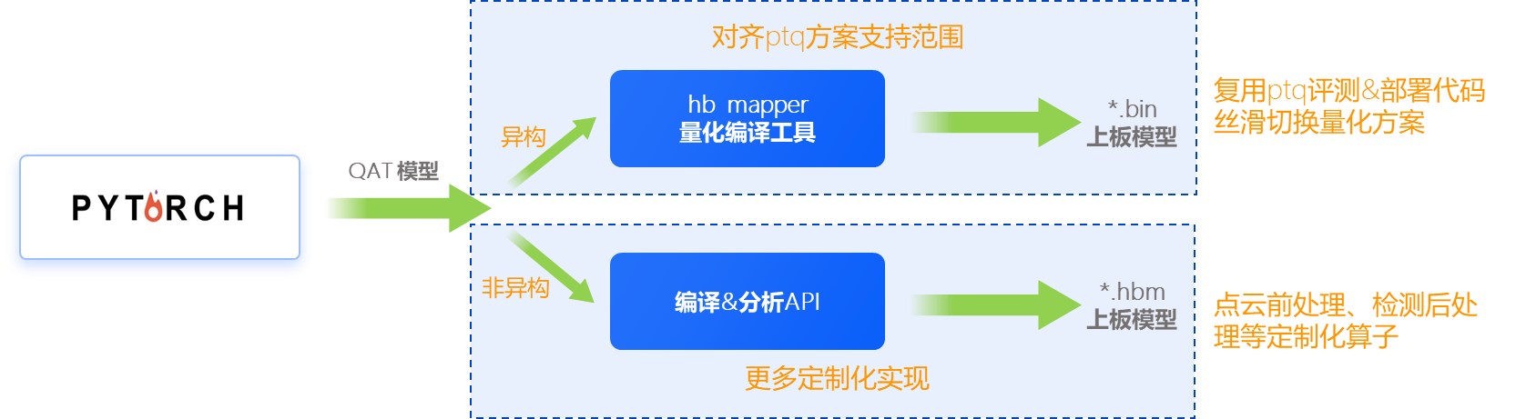
其中第一种异构方案的编译及部署方式与PTQ方案完全对齐，就不再赘述了，后文讨论的均是非异构方案。

第二种非异构方案是直接调用python API完成模型转换编译，最终生成的是.hbm后缀的模型，该模型由纯bpu指令组成，因此量化/反量化等cpu操作都需要用户自行在前后处理里完成。

2.1 与模型输入/输出信息相关的配置项

编译模型使用的API为compile_model，支持的配置选项如下：

def compile_model( 
        module: Union[torch.jit.ScriptModule, torch.nn.Module],  
        example_inputs: tuple, 
        hbm: str, 
        march: str = None, 
        name: str = None, 
 input_source: Union[Sequence[str], str] = "ddr", # Specify input features' sources(ddr/resizer/pyramid). 
 input_layout: str = None, #  Specify input layout of all model inputs.Available layouts are NHWC, NCHW 
 output_layout: str = "NCHW", 
        opt: Union[str, int] = "O2", 
        jobs: int = 16, 
        debug: bool = False, 
        extra_args: list = None, # specify extra args listed in "hbdk-cc -h" 
): 

该API只有input_source以及input_layout参数与模型输入信息相关（与PTQ方案中的编译参数组compiler_parameters相对应），因此缺少了预处理节点相关配置项。若想将图像格式转换（rgb、bgr转yuv）以及归一化操作放到模型中使用硬件加速的话，请参考下一节 2.2 camera输入注意事项

2.2 camera输入注意事项

同样的，我们依然以yolov5s模型为例，说明camera输入场景下如何将图像格式转换以及归一化操作配置进模型中实现硬件加速。（yolov5s浮点训练的预处理代码请参考前文1.2节）

2.2.1 模型转换

plugin通过开发了两个预处理算子用于实现yuv444到rgb/bgr的转换以及归一化操作的硬件加速。这两个算子分别为centered_yuv2rgb以及centered_yuv2bgr。算子定义：

def centered_yuv2rgb( 
    input: QTensor, 
    swing: str = "studio", # "studio" for YUV studio swing (Y: -112~107,U, V: -112~112)；"full" for YUV full swing (Y, U, V: -128~127)；mipi摄像机选择full，bt601_video选择studio 
    mean: Tensor = torch.tensor([128.0]), # rgb mean, a scalar tensor or a tensor of size [3] 
    std: Tensor = torch.tensor([128.0]), # rgb standard deviation, a scalar tensor or a tensor of size [3] 
    q_scale: Tensor = torch.tensor([1.0 / 128.0]), # rgb quantization scale. must be scalar tensor 
) -> QTensor: 

该算子为纯定点算子，不参与模型训练的过程。该算子使用方式如下：

1. 通过QAT训练得到满意的精度之后，先使用convert()接口将qat模型转为quantized模型；
2. 修改forward，在QuantStub后插入该算子；
3. 设置QuantStub的scale=1（因为QuantStub已经被合入到了centered_yuv2rgb中，此处只有标识符的作用）；
4. 推理一次quantized模型。

参考代码：

import torch 
import horizon_plugin_pytorch as horizon 
from horizon_plugin_pytorch.functional import centered_yuv2rgb 
 
class Net(torch.nn.Module): 
    def __init__(self): 
        super().__init__() 
        self.quant = hz.quantization.QuantStub(scale=1.0) 
        self.convnet = ConvNet() 
 
    def forward(self, input): 
        x = self.quant(input) 
        x = centered_yuv2rgb( 
            x, 
            mean=torch.tensor([0]), 
            std=torch.tensor([255]), # yolov5模型的数据归一化仅包含了/255的操作 
            q_scale=torch.tensor([1 / 128]), # 默认值为1/128，若训练时使用了动态QuantStub，则需要设置为observe的scale值 
        ) 
        x = self.convnet(x) 
        return x 

可通过print model或visualize_model()观察是否已插入该算子。

若模型使用yuv444格式训练，建议数据归一化操作为减128并除以128，同时需要将QuantStub的scale设置为1/128。 编译模型时注意设置input_source为pyramid。与ptq有所不同的是，大家会发现编译出来的hbm模型在板端解析出来其输入数据类型不是HB_DNN_IMG_TYPE_NV12，而是HB_DNN_IMG_TYPE_NV12_SEPARATE，后者的y和uv分量是分别存储的，需要为其申请两个hbSysMem，这也是由于pyramid出来的数据是y和uv分量分开存储的两个地址，因此该数据类型更方便分开为y和uv赋值。

2.2.2 PC端与板端推理一致性验证

在PC端验证quantized模型精度时需要在预处理阶段完成rgb/bgr转nv12+nv12转yuv444的过程，具体原因请参考前文 1.2.2 节。

1. quantized模型（或是traced模型）推理示例代码：

import cv2 
import numpy as np 
from PIL import Image 
import horizon_plugin_pytorch as horizon 
 
# note: image.shape = (h, w, c) 
# nv12数据与YUV_I420的uv分量排列方式不同，具体请参考用户手册BPU SDK API文档的NV12介绍 
def bgr2nv12(image): 
    image = image.astype(np.uint8) 
    height, width = image.shape[0], image.shape[1] 
    yuv420p = cv2.cvtColor(image, cv2.COLOR_BGR2YUV_I420).reshape((height * width * 3 // 2, )) 
    y = yuv420p[:height * width] 
    uv_planar = yuv420p[height * width:].reshape((2, height * width // 4)) 
    uv_packed = uv_planar.transpose((1, 0)).reshape((height * width // 2, )) 
    nv12 = np.zeros_like(yuv420p) 
    nv12[:height * width] = y 
    nv12[height * width:] = uv_packed 
    return nv12 
 
def nv12Toyuv444(nv12, target_size): 
    height = target_size[0] 
    width = target_size[1] 
    nv12_data = nv12.flatten() 
    yuv444 = np.empty([height, width, 3], dtype=np.uint8) 
    yuv444[:, :, 0] = nv12_data[:width * height].reshape(height, width) 
    u = nv12_data[width * height::2].reshape(height // 2, width // 2) 
    yuv444[:, :, 1] = Image.fromarray(u).resize((width, height),resample=0) 
    v = nv12_data[width * height + 1::2].reshape(height // 2, width // 2) 
    yuv444[:, :, 2] = Image.fromarray(v).resize((width, height),resample=0) 
    return yuv444 
 
def preprocess(): 
    img = cv2.imread("1.jpg") 
    # 测精度时需要使用padresize，为了缩减代码篇幅，因此此处仅使用resize 
    img = cv2.resize(img,(672,672))  
    # 处理至input_type_rt中间类型 
    nv12 = bgr2nv12(img) 
    # .hbm模型的输入数据 
    nv12.tofile("nv12_data_yolov5s.bin") 
    # nv12 to yuv444_128 
    img = nv12Toyuv444(nv12, (672,672)).astype(np.float32) 
    img = img[np.newaxis,:,:,:] -128.0
    return img 
 
quantized_model = horizon.quantization.convert(qat_model.eval(), inplace=False) 
img = preprocess() 
img = img.permute((0, 3, 1, 2)) 
quantized_model = quantized_model.cpu() 
output = quantized_model(img) 
print(outputs[0]) 

2. hbm模型快速验证：

若仅做一致性验证，推荐使用hrt_model_exec infer工具，无需任何代码开发，按照前文参考代码，在Python端准备好nv12数据即可。

hrt_model_exec infer --model_file yolov5s.hbm --input_file nv12_data_yolov5s.bin --enable_dump 1 --dump_format txt 

由于hbm模型不包含量化/反量化等cpu操作，因此hbm模型输出为定点数，需要自行在后处理逻辑中完成反量化操作，C++示例代码请参考反量化节点的融合实现。

此外，由于硬件有stride要求，因此大家还需要注意在前后处理代码中完成padding和remove padding的操作，具体解析请参考模型输入输出对齐规则解析。

2.3 featuremap输入注意事项

featuremap即input_source=ddr的模型，由于hbm模型不包含量化/反量化等cpu操作，因此该部分均需用户自行在前后处理中完成，C++示例代码请参考反量化节点的融合实现。

此外，由于硬件有stride要求，因此大家还需要注意在前后处理代码中完成padding和remove padding的操作，具体解析请参考模型输入输出对齐规则解析。

3 其他应用开发技巧

batch模型

文档：多batch模型使用与部署

crop/resize加速

方案一：使用VPS，支持对图像进行缩小、放大、裁剪、旋转、GDC矫正、帧率控制以及金字塔图像输出（相关介绍文档，J3/J5用户请联系项目对接人获取，x3用户可查阅在线手册）

方案二：使用RoiInfer接口实现corp+resize(硬件加速） （文档：resizer模型使用与部署）

多模型批处理 (减少中断耗时)

示例：OE:/ddk/samples/ai_toolchain/horizon_runtime_sample/code/02_advanced_samples/multi_model_batch

文档：工具链用户手册《BPU SDK API》

优先级调度

文档：工具链用户手册应用开发章节-模型优先级控制

[寒山不冷]

PTQ是以后的版本也不能编译出HB_DNN_IMG_TYPE_NV12_SEPARATE格式的模型吗？