0 概述-
在自动驾驶感知算法中BEV感知成为热点话题,BEV感知可以弥补2D感知的缺陷构建3D“世界”,更有利于下游任务和特征融合。为响应市场需求,地平线集成了基于bev的纯视觉算法,目前已支持ipm-based 、lss-based、 transformer-based(Geometry-guided Kernel Transformer、detr3d) 的多种bev视觉转换方法。本文为ipm-based的BEV多任务感知算法介绍和使用说明。-
该示例为参考算法,仅作为在J5上模型部署的设计参考,非量产算法
1 性能精度指标-
模型配置:-
数据集
img_shape
backbone
grid_size
Nuscenes
512 x 960
efficientnetb0
128x128
性能精度表现:
性能(FPS/单核)
分割精度
检测精度(NDS)
106
51.45/51.45
0.3060/0.3068
注:stage1为image encoder;stage2为bev encoder-
Nuscenes 数据集官方介绍:https://www.nuscenes.org/nuscenes#overview
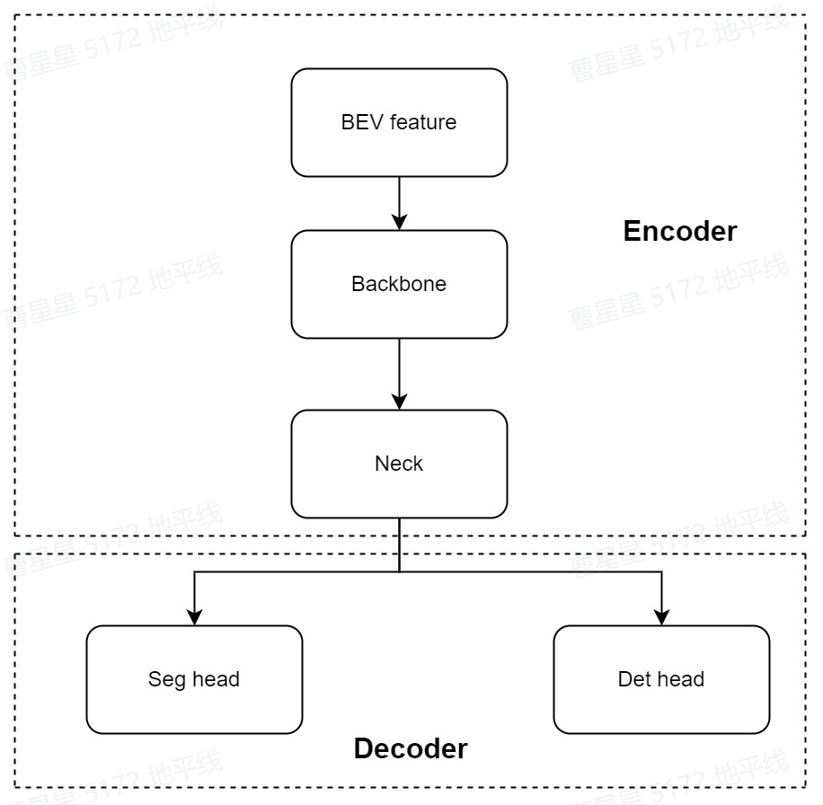
2 模型介绍
2.1 模型框架
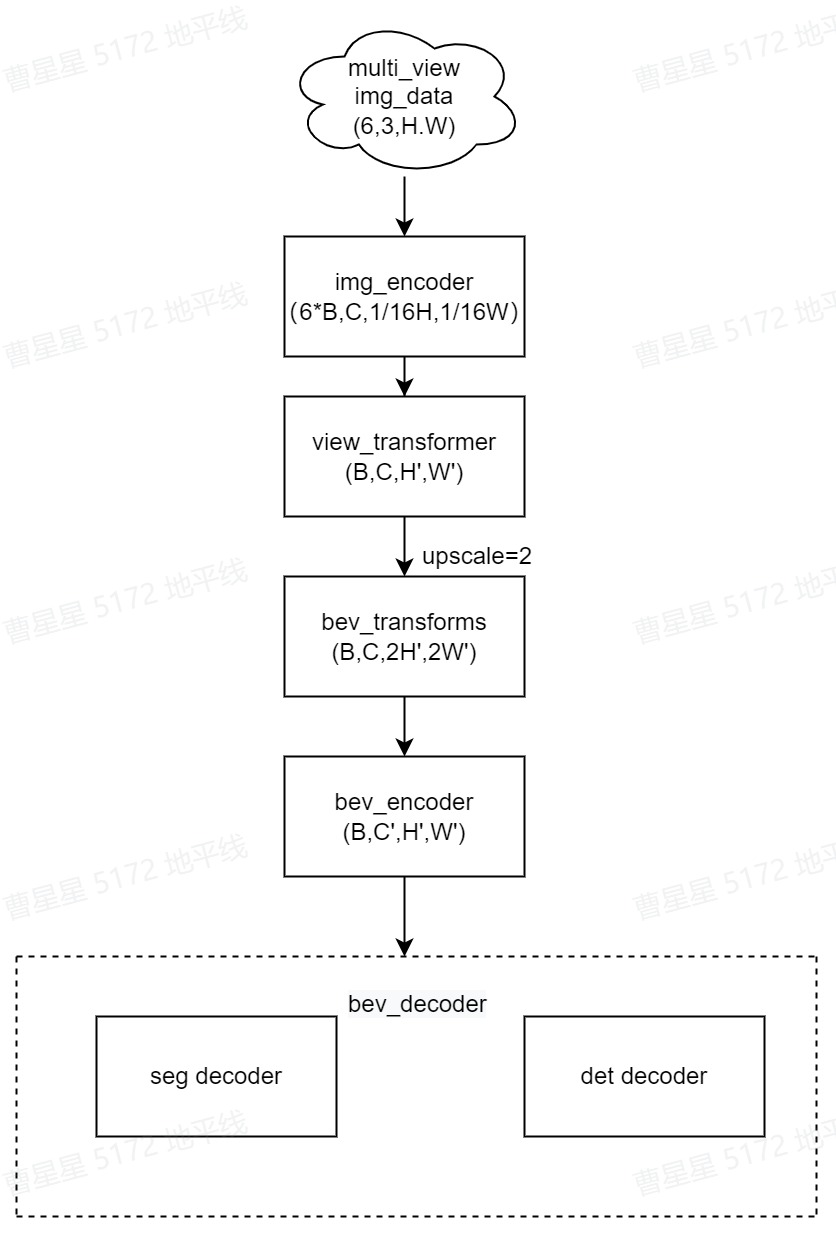
bev_ipm 使用多视图的当前帧的6个RGB图像作为输入。输出是目标的3D Box和BEV分割结果。多视角图像首先使用2D主干获取2D特征。然后投影到3D BEV视角。接着对BEV feature 编码获取BEV特征。最后,接上任务特定的head,输出多任务结果。模型主要包括以下部分:-
**Part1—2D Image Encoder:**图像特征提取层。使用2D主干网络(efficientnet)和FastSCNN输出不同分辨率的特征图。返回最后一层–下采样至1/16原图大小层,用于下一步投影至3D 坐标系中。-
**Part2—View transformer:**采用IPM映射完成img 2D到bev 3D的转换。-
**Part3—Bev transforms:**对bev特征做数据增强,仅发生在训练阶段。-
**Part4—3D BEV Encoder:**BEV特征提取层。-
**Part5—BEV Decoder:**分为Detection Head和Segmentation Head。得到统一的BEV特征后,使用DepthwiseSeparableFCNHead进行bev分割,分割种类为[“others”, “divider”, “ped_crossing”, “Boundary”]。使用DepthwiseSeparableCenterPointHead进行3D目标检测任务,检测的类别为[“car”,“truck”,“bus”,“barrier”,“bicycle”,“pedestrian”]。-
2.2 源码说明-
Config文件-
configs/bev/bev_ipm_efficientnetb0_multitask_nuscenes.py 为该模型的配置文件,定义了模型结构、数据集加载,和整套训练流程,所需参数的说明在算子定义中会给出。配置文件主要内容包括:-
#基础参数配置
task_name = "bev_ipm_efficientnetb0_multitask_nuscenes"
batch_size_per_gpu = 2
device_ids = [0]
#bev参数配置
data_shape = (3, 512, 960)
bev_size = (51.2, 51.2, 0.8)
map_size = (15, 30, 0.15)

# 模型结构定义
model = dict(
    type="ViewFusion",
    backbone=dict(
        type="efficientnet",
        model_type="b0",
        ...
    ),
    neck=dict(
        type="FastSCNNNeck",
        ...
    ),
    view_transformer=dict(
        type="WrappingTransformer", #ipm transform
        ...
    ),
    bev_transforms=[...],
    bev_encoder=dict(
        type="BevEncoder",
        ...
    ),
    bev_decoders=[
        dict(
            type="BevSegDecoder",
            ...
         ),
         dict(
            type="BevDetDecoder",
            ...
        )
    ],
)

deploy_model = dict(
...
)
...
# 数据加载
data_loader = dict(
    type=torch.utils.data.DataLoader,
    ...
)

val_data_loader = dict(...)

#不同step的训练策略配置
float_trainer=dict(...)
calibration_trainer=dict(...)
int_infer_trainer=dict(...)
#不同step的验证
float_predictor=dict(...)
calibration_predictor=dict(...)
int_infer_predictor=dict(...)
#编译配置
compile_cfg = dict(
    march=march,
    ...
)
注: 如果需要复现精度,config中的训练策略最好不要修改。否则可能会有意外的训练情况出现。
img_encoder
来自6个view的image作为输入通过共享的backbone(efficientnet)和neck(FastSCNN)输出经过encoder后的feature,feature_shape为(6*B,C,1/16H,1/16W)。encoder即对多个view的img_feature 做特征提取,过程见下图:

对应代码:hat/models/backbones/efficientnet.py hat/models/necks/fast_scnn.py-
view_transformer-
view_transformer 采用IPM映射的方法,基于摄像头的内外参把图像视角的img_features转换到bev_features。bev_shape为[H’,W’]为[128,128],其转换过程见下图:
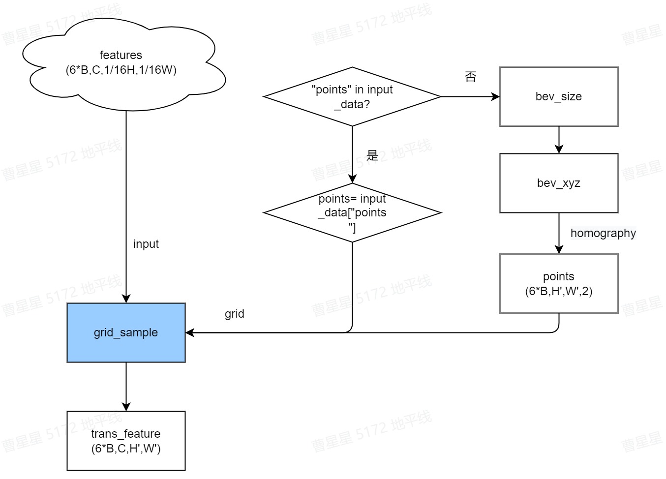
view_transformer对应代码:hat/models/task_modules/view_fusion/view_transformer.py 的 WrappingTransformer
class WrappingTransformer(ViewTransformer):
    ...
    def _spatial_transfom(self, feat, points):
        if isinstance(points, placeholder):
            points = points.sample
        #[nview*B, C, 1/16H, 1/16W]-->#([nview*B, C, 128, 128]
        trans_feats = self.grid_sample(
            feat,
            self.quant_stub(points),
        )
        ...

        return fused_feats
其中,grid_sample在plugin中实现,路径为:horizon_plugin_pytorch/nn/grid_sample.py
def forward(self, x, grid):
    # type: (Tensor, Tensor) -> Tensor
    """
    Forward pass of GridSample.

    Args:
        x (Tensor[N, C, H, W]): Input data.
        grid (Tensor[N, H_out, W_out, (dx, dy)]): Flow-field. This param
            is different with torch.nn.functional.grid_sample. In this
            function, the sample point of output point (x, y) is computed
            by (x + dx, y + dy).
    """
    # convert grid format from 'delta' to 'norm'
    n = grid.size(0)
    h = grid.size(1)
    w = grid.size(2)
    base_coord_y = (
        torch.arange(h, dtype=grid.dtype, device=grid.device)
        .unsqueeze(-1)
        .unsqueeze(0)
        .expand(n, h, w)
    )
    base_coord_x = (
        torch.arange(w, dtype=grid.dtype, device=grid.device)
        .unsqueeze(0)
        .unsqueeze(0)
        .expand(n, h, w)
    )
    absolute_grid_x = grid[:, :, :, 0] + base_coord_x
    absolute_grid_y = grid[:, :, :, 1] + base_coord_y
    norm_grid_x = absolute_grid_x * 2 / (x.size(3) - 1) - 1
    norm_grid_y = absolute_grid_y * 2 / (x.size(2) - 1) - 1
    norm_grid = torch.stack((norm_grid_x, norm_grid_y), dim=-1)

    r = F.grid_sample(x, norm_grid, self.mode, self.padding_mode, True)
    return r
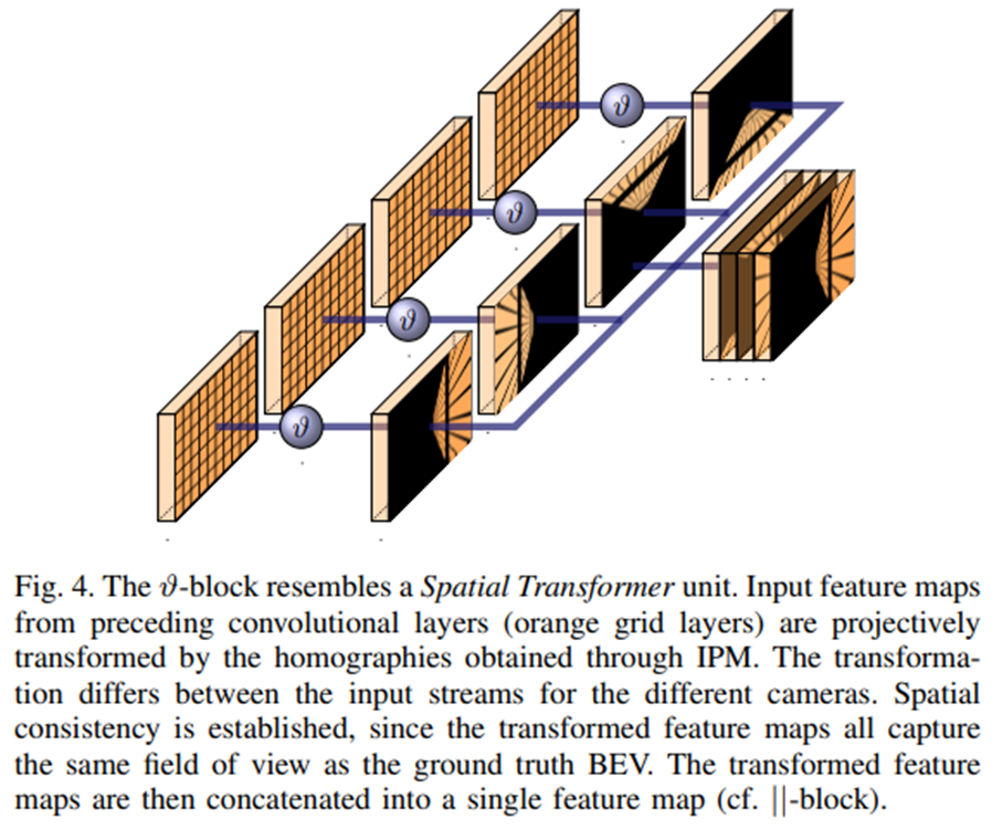
spatial_transfomer-
grid_sample的输入为多个view的img feature,经过bev 转换后将进行多view的特征融合,如下图所示:
对应代码为:
if self.training or batch_size > 1:
    trans_feats = trans_feats.view(
        batch_size,
        self.num_views,
        trans_feats.shape[1],
        trans_feats.shape[2],
        trans_feats.shape[3],
    )
    #多view 特征融合
    fused_feats = self.floatFs.sum(trans_feats, keepdim=True, dim=1)
    fused_feats = fused_feats.view(
        batch_size,
        trans_feats.shape[2],
        trans_feats.shape[3],
        trans_feats.shape[4],
    )
else:
    fused_feats = self.floatFs.sum(trans_feats, keepdim=True, dim=0)
homography矩阵
homography矩阵是将相机视角转换成鸟瞰图的关键所在,计算方式为:
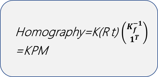
对于Kf:
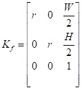
其中,K为相机内参; P为相机外参即(R, t)为转换角和偏移; M为bev坐标到世界坐标的转换矩阵,(W, H)为bev的长度和宽度,r为1m的像素数。-
对应代码:hat/models/task_modules/view_fusion/view_transformer.py
def _get_homography(self, meta, feats):
    homography = meta["ego2img"]
    feat_hw = feats.shape[2:]
    orig_hw = meta["img"][0].shape[1:]
    scales = (feat_hw[0] / orig_hw[0], feat_hw[1] / orig_hw[1])
    view = np.eye(4)
    view[0, 0] = scales[1]
    view[1, 1] = scales[0]
    view = torch.tensor(view).to(device=homography.device)
    homography = torch.matmul(view, homography)
    return homography
通过homo转换为像素坐标中的coors,对应代码:
def _gen_reference_point(self, homography, feats=None):
    ...
    for homo in homography:
        new_coord = torch.matmul(coords, homo.permute((1, 0)))
        new_coords.append(new_coord)
bev transform-
bev的数据增强仅发生在训练过程中,在 BEV 下做了 rotate的数据增强,作用域是 view transformer 的输出。配置如下:
bev_transforms=[
    dict(
        type="BevRotate",
        bev_size=bev_size,
        rot=(-0.3925, 0.3925),
    ),
],
bev_encoder-
bev_encoder过程是对bev_feature 做特征提取的过程,backbone为efficientnet-b0,neck为BiFPN。流程见下图:
对应代码:hat/models/task_modules/view_fusion/encoder.py
class BevEncoder(nn.Module):
    def __init__(self, backbone: nn.Module, neck: nn.Module):
        super(BevEncoder, self).__init__()
        self.backbone = backbone
        self.neck = neck

    def forward(self, feat, meta):
        feat = self.backbone(feat)
        if self.neck is not None:
            feat = self.neck(feat)
        return feat
bev_head-
seg_head-
本模型的分割头为DepthwiseSeparableFCNHead,conv为SeparableConvModule2d-
对应代码:hat/models/task_modules/fcn/head.py
class DepthwiseSeparableFCNHead(FCNHead):
    def __init__(self, in_channels, feat_channels, num_convs=1, **kwargs):

        super(DepthwiseSeparableFCNHead, self).__init__(
            in_channels=in_channels, feat_channels=feat_channels, **kwargs
        )
        self.convs = nn.Sequential(
            SeparableConvModule2d(
                in_channels,
                ...
                dw_norm_layer=nn.BatchNorm2d(
                ),
            ),

class FCNHead(nn.Module):
    def __init__(self,...):
    ...
    def forward(self, inputs: List[torch.Tensor]):
        x = inputs[self.input_index]
        x = self.convs(x)
        if self.dropout:
            x = self.dropout(x)
        seg_pred = self.cls_seg(x)
        if self.training:
            if self.upsample_output_scale:
                seg_pred = self.resize(seg_pred)
            if self.argmax_output:
                seg_pred = seg_pred.argmax(dim=1)
        if self.dequant_output:
            seg_pred = self.dequant(seg_pred)
        return seg_pred
det_head
检测为多task检测,主要分为:
tasks = [
    dict(name="car", num_class=1, class_names=["car"]),
    dict(
        name="truck",
        num_class=2,
        class_names=["truck", "construction_vehicle"],
    ),
    dict(name="bus", num_class=2, class_names=["bus", "trailer"]),
    dict(name="barrier", num_class=1, class_names=["barrier"]),
    dict(name="bicycle", num_class=2, class_names=["motorcycle", "bicycle"]),
    dict(
        name="pedestrian",
        num_class=2,
        class_names=["pedestrian", "traffic_cone"],
    ),
]
在nuscenes数据集中,目标的类别一共被分为了6个大类,网络给每一个类都分配了一个head,装在headlist中,而每个head内部都为预测的参数。-
bev_det的分割头为DepthwiseSeparableCenterPointHead-
对应代码:hat/models/task_modules/centerpoint/head.py
class DepthwiseSeparableCenterPointHead(CenterPointHead):
    def _make_conv(
        self,
        ...
    ):
        pw_norm_layer = nn.BatchNorm2d(in_channels, **self.bn_kwargs)
        pw_act_layer = nn.ReLU(inplace=True)

        return SeparableConvModule2d(
            in_channels=in_channels,
            ...
        )

    def _make_task(self, **kwargs):
        return DepthwiseSeparableTaskHead(**kwargs)

class CenterPointHead(nn.Module):
    def __init__(self,...):
        self.shared_conv = nn.Sequential(
            *(
                self._make_conv(
                    in_channels=in_channels if i == 0 else share_conv_channels,
                    ...
                )
                for i in range(share_conv_num)
            )
        )
        #head module
        for num_cls in num_classes:
            heads = copy.deepcopy(common_heads)
            heads.update({"heatmap": (num_cls, num_heatmap_convs)})
            task_head = self._make_task(
                ...,
            )
            self.task_heads.append(task_head)

    def forward(self, feats):
        rets = []
        feats = feats[0]
        feats = self.shared_conv(feats)
        for task in self.task_heads:
            rets.append(task(feats))
forward时,经过共享的SeparableConv后,将feature再分别传入task_heads做task_pred。-
在hat/models/task_modules/centerpoint/head.py的TaskHead对不同的task定义conv_layers:
class DepthwiseSeparableTaskHead(TaskHead):
    def _make_conv(
        self,
        in_channels,
        ...
    ):
        return SeparableConvModule2d(
            in_channels=in_channels,
            ...
        )

class TaskHead(nn.Module):
    def __init__(...):
         ...
         for head in self.heads:
            classes, num_conv = self.heads[head]
            ...
            #head_conv
            for _ in range(num_conv - 1):
                conv_layers.append(
                    self._make_conv(
                    ...
                    )
                )
                c_in = head_conv_channels
            #cls_layer
            conv_layers.append(
                ConvModule2d(
                    in_channels=head_conv_channels,
                    out_channels=classes,
                    ...
                )
            )
            conv_layers = nn.Sequential(*conv_layers)

    def forward(self, x):
        ret_dict = {}
        for head in self.heads:
            ret_dict[head] = self.dequant(self.__getattr__(head)(x))
        return ret_dict
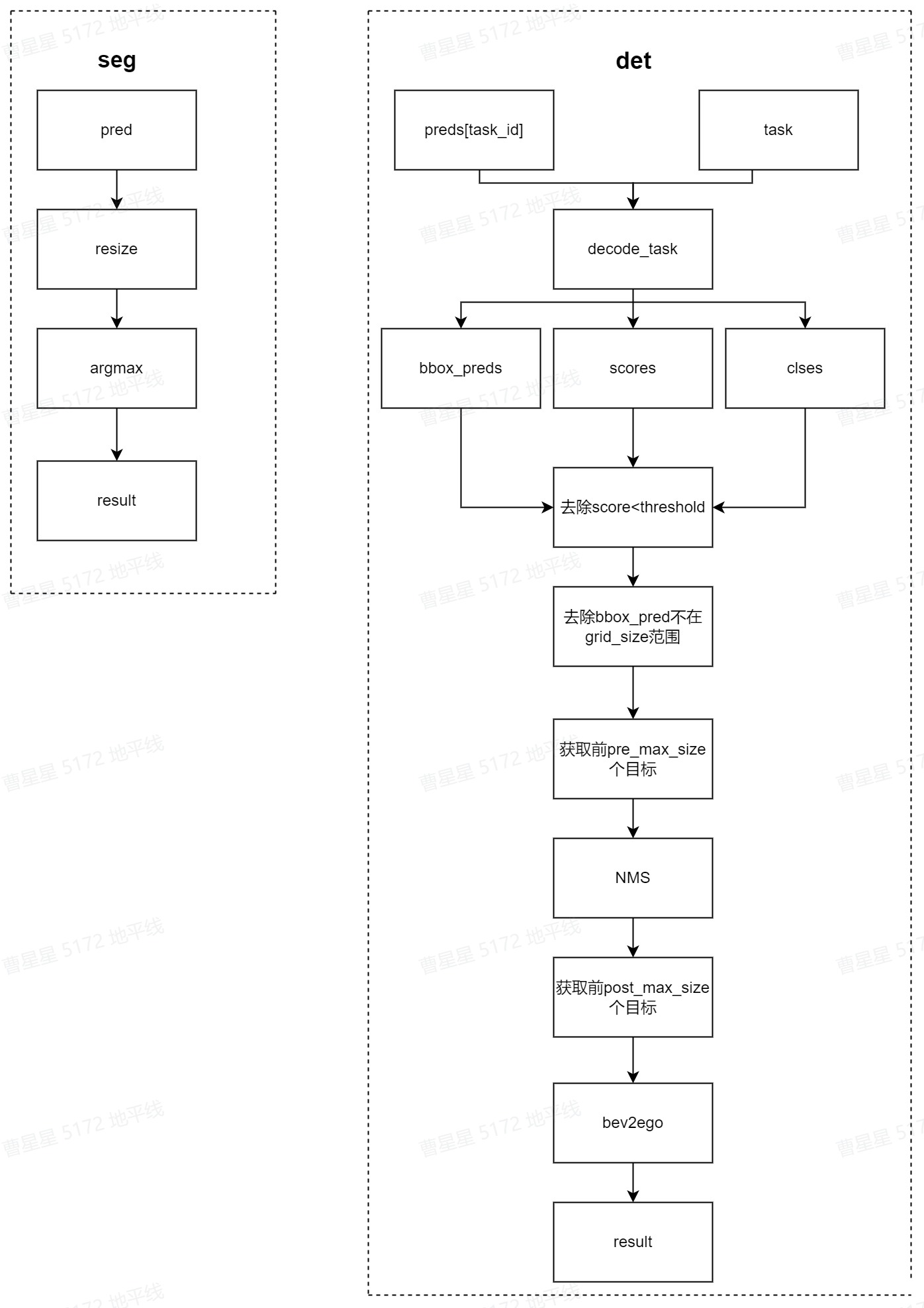
bev_decoder-
多任务模型的decoder分为分割和检测的解码,在分割任务中使用FCNDecoder,在检测任务中使用CenterPointDecoder,具体实现流程见下图:
对应代码:-
hat/models/task_modules/centerpoint/decoder.py-
hat/models/task_modules/fcn/decoder.py-
3 浮点模型训练-
3.1 Before Start-
3.1.1 发布物及环境部署-
step1:获取发布物-
下载OE包horizon_j5_open_explorer_v$version$.tar.gz,获取方式见地平线开发者社区 OpenExplorer算法工具链 版本发布-
step2:解压发布包
tar -xzvf horizon_j5_open_explorer_v$version$.tar.gz
解压后文件结构如下:
|-- bsp
|-- ddk
|   |-- package
|   `-- samples
|       |-- ai_benchmark
|       |-- ai_forward_view_sample
|       |-- ai_toolchain
|       |   |-- ...
|       |   |-- horizon_model_train_sample
|       |   `-- model_zoo
|       |-- model_zoo
|       `-- vdsp_rpc_sample
|-- README-CN
|-- README-EN
|-- resolve_all.sh
`-- run_docker.sh
其中horizon_model_train_sample为参考算法模块,包含以下模块:
|-- horizon_model_train_sample  #参考算法示例
|   |-- plugin_basic  #qat 基础示例
|   `-- scripts  #模型配置文件、运行脚本
step3:拉取docker环境
docker pull openexplorer/ai_toolchain_ubuntu_20_j5_gpu:v$version$
#启动容器,具体参数可根据实际需求配置
#-v 用于将本地的路径挂载到 docker 路径下
nvidia-docker run -it --shm-size="15g" -v `pwd`:/WORKSPACE openexplorer/ai_toolchain_ubuntu_20_j5_gpu:v$version$
3.1.2 数据集准备-
3.1.2.1 数据集下载-
进入nuscenes官网,根据提示完成账户的注册,下载Full dataset(v1.0)、CAN bus expansion和Map expansion(v1.3)这三个项目下的文件。下载后的压缩文件为:
|-- nuScenes-map-expansion-v1.3.zip
|-- can_bus.zip
|-- v1.0-mini.tar
|-- v1.0-trainval01_blobs.tar
|-- ...
|-- v1.0-trainval10_blobs.tar
`-- v1.0-trainval_meta.tar
Full dataset(v1.0)包含多个子数据集,如果不需要进行v1.0-trainval数据集的浮点训练和精度验证,可以只下载v1.0-mini数据集进行小场景的训练和验证。
将下载完成的v1.0-trainval01_blobs.tar~v1.0-trainval10_blobs.tar、v1.0-trainval_meta.tar和can_bus.zip进行解压,解压后的目录如下所示:
|--nuscenes
    |-- can_bus #can_bus.zip解压后的目录
    |-- samples #v1.0-trainvalXX_blobs.tar解压后的目录
    |   |-- CAM_BACK
    |   |-- ...
    |   |-- CAM_FRONT_RIGHT
    |   |--  ...
    |   `-- RADAR_FRONT_RIGHT
    |-- sweeps
    |   |-- CAM_BACK
    |   |-- ...
    |   |-- CAM_FRONT_RIGHT
    |   |--  ...
    |   `-- RADAR_FRONT_RIGHT
    |-- v1.0-trainval #v1.0-trainval_meta.tar解压后的数据
        |-- attribute.json
        |    ...
        `-- visibility.json
3.1.2.2 数据集打包-
进入 horizon_model_train_sample/scripts 目录,使用以下命令将训练数据集和验证数据集打包,格式为lmdb:
#pack train_Set
python3 tools/datasets/nuscenes_packer.py --src-data-dir /WORKSPACE/nuscenes/ --pack-type lmdb --target-data-dir /WORKSPACE/tmp_data/nuscenes/v1.0-trainval --version v1.0-trainval --split-name train
#pack val_Set
python3 tools/datasets/nuscenes_packer.py --src-data-dir /WORKSPACE/nuscenes/ --pack-type lmdb --target-data-dir /WORKSPACE/tmp_data/nuscenes/v1.0-trainval --version v1.0-trainval --split-name val
--src-data-dir为解压后的nuscenes数据集目录;-
--target-data-dir为打包后数据集的存储目录;-
--version 选项为[“v1.0-trainval”, “v1.0-test”, “v1.0-mini”],如果进行全量训练和验证设置为v1.0-trainval,如果仅想了解模型的训练和验证过程,则可以使用v1.0-mini数据集;v1.0-test数据集仅为测试场景,未提供注释。-
全量的nuscenes数据集较大,打包时间较长。每打包完100张会在终端有打印提示,其中train打包约28100张,val打包约6000张。
数据集打包命令执行完毕后会在target-data-dir下生成train_lmdb和val_lmdb,train_lmdb和val_lmdb就是打包之后的训练数据集和验证数据集为config中的data_rootdir。
|-- tmp_data
|   |-- nuscenes
|   |   |-- v1.0-trainval
|   |   |   |-- train_lmdb  #打包后的train数据集
|   |   |   |   |-- data.mdb
|   |   |   |   `-- lock.mdb
|   |   |   `-- val_lmdb   #打包后的val数据集
|   |   |   |   |-- data.mdb
|   |   |   |   `-- lock.mdb
2.1.2.3 meta文件夹构建-
在tmp_data/nuscenes 下创建meta文件夹,将v1.0-trainval_meta.tar压缩包解压至meta,得到meta/maps文件夹,再将nuScenes-map-expansion-v1.3.zip压缩包解压至meta/maps文件夹下,解压后的目录结构为:
|-- tmp_data
|   |-- nuscenes
|   |   |-- meta
|   |   |   |-- maps        #nuScenes-map-expansion-v1.3.zip解压后的目录
|   |   |   |   |-- 36092f0b03a857c6a3403e25b4b7aab3.png
|   |   |   |   |-- ...
|   |   |   |   |-- 93406b464a165eaba6d9de76ca09f5da.png
|   |   |   |   |-- prediction
|   |   |   |   |-- basemap
|   |   |   |   |-- expansion
|   |   |   |-- v1.0-trainval  #v1.0-trainval_meta.tar解压后的目录
|   |   |       |-- attribute.json
|   |   |           ...
|   |   |       |-- visibility.json
|   |   `-- v1.0-trainval
|   |   |   |-- train_lmdb  #打包后的train数据集
|   |   |   `-- val_lmdb   #打包后的val数据集
3.1.3 config配置-
在进行模型训练和验证之前,需要对configs文件中的部分参数进行配置,一般情况下,我们需要配置以下参数:
- device_ids、batch_size_per_gpu:根据实际硬件配置进行device_ids和每个gpu的batchsize的配置;
- ckpt_dir:浮点、calib、量化训练的权重路径配置,权重下载链接在config文件夹下的README中;
- data_rootdir:2.1.2.2中打包的数据集路径配置;
- meta_rootdir :2.1.2.3中创建的meta文件夹的路径配置;
- float_trainer下的checkpoint_path:浮点训练时backbone的预训练权重所在路径,可以使用README的# Backbone Pretrained ckpt中ckpt download提供的float-checkpoint-best.pth.tar权重文件。
- infer_cfg:指定模型输入,在infer.py脚本使用时需配置;
3.2 浮点模型训练-
config文件中的参数配置完成后,使用以下命令训练浮点模型:
python3 tools/train.py --config configs/bev/bev_ipm_efficientnetb0_multitask_nuscenes.py --stage float
float训练后模型ckpt的保存路径为config配置的
ckpt_callback中save_dir的值,默认为ckpt_dir。
3.3 浮点模型精度验证-
浮点模型训练完成以后,通过指定训好的float_checkpoint_path,使用以下命令验证已经训练好的模型精度:
python3 tools/predict.py --config configs/bev/bev_ipm_efficientnetb0_multitask_nuscenes.py --stage float
验证完成后,会在终端打印浮点模型在验证集上检测和分割精度,如下所示:
Per-class results:
Object Class    AP      ATE     ASE     AOE     AVE     AAE
car     0.416   0.571   0.184   0.400   1.329   0.209
...
2023-06-06 18:24:09,976 INFO [nuscenes_metric.py:358] Node[0] NDS: 0.3060, mAP:0.2170
...
2023-06-06 18:24:10,513 INFO [mean_iou.py:170] Node[0] ~~~~ MeanIOU Summary metrics ~~~~
Summary:
Scope                 mIoU       mAcc       aAcc
global               51.47      75.62      86.29
Per Class Results:
Class                  IoU        Acc
others               85.10      88.42
...
2023-06-06 18:24:10,524 INFO [metric_updater.py:320] Node[0] Epoch[0] Validation bev_ipm: NDS[0.3060] MeanIOU[tensor(0.5147, device='cuda:0')]
4 模型量化和编译-
完成浮点训练后,还需要进行量化训练和编译,才能将定点模型部署到板端。地平线对该模型的量化采用horizon_plugin框架,经过Calibration+定点模型转换后,使用compile的工具将量化模型编译成可以上板运行的hbm文件。-
4.1 Calibration-
模型完成浮点训练后,便可进行 Calibration。calibration在forward过程中通过统计各处的数据分布情况,从而计算出合理的量化参数。 通过运行下面的脚本就可以开启模型的Calibration过程:
python3 tools/train.py --config configs/bev/bev_ipm_efficientnetb0_multitask_nuscenes.py --stage calibration
4.2 Calibration 模型精度验证-
calibration完成以后,可以使用以下命令验证经过calib后模型的精度:
python3 tools/predict.py --config configs/bev/bev_ipm_efficientnetb0_multitask_nuscenes.py --stage calibration
验证完成后,会在终端输出calib模型在验证集上检测和分割精度,格式见3.3。-
对于IPM模型,仅需做calib 即可满足量化精度,无需做qat训练!
4.3 量化模型精度验证-
指定calibration-checkpoint后,通过运行以下命令进行量化模型的精度验证:
python3 tools/predict.py --config configs/bev/bev_ipm_efficientnetb0_multitask_nuscenes.py --stage int_infer
验证完成后,会在终端输出int模型在验证集上检测和分割精度,格式见3.3。
4.4 仿真上板精度验证-
除了上述模型验证之外,我们还提供和上板完全一致的精度验证方法,可以通过下面的方式完成:
python3 tools/align_bpu_validation.py --config configs/bev/bev_ipm_efficientnetb0_multitask_nuscenes.py
4.5 量化模型编译-
在训练完成之后,可以使用compile的工具用来将量化模型编译成可以上板运行的hbm文件,同时该工具也能预估在BPU上的运行性能,可以采用以下脚本:
python3 tools/compile_perf.py --config configs/bev/bev_ipm_efficientnetb0_multitask_nuscenes.py --out-dir ./ --opt 3
--opt为优化等级,取值范围为0~3,数字越大优化等级越高,编译时间也会越长;-
可以指定–out_dir为编译后产出物的存放路径,默认在ckpt_dir的compile文件夹下
运行后,ckpt_dir的compile目录下会产出以下文件:
|-- compile
|   |-- .html #模型在bpu上的静态性能数据
|   |-- .json
|   |-- model.hbm  #板端部署的模型
|   |-- model.hbir #编译过程的中间文件
    `-- model.pt   #模型的pt文件
5 其他工具-
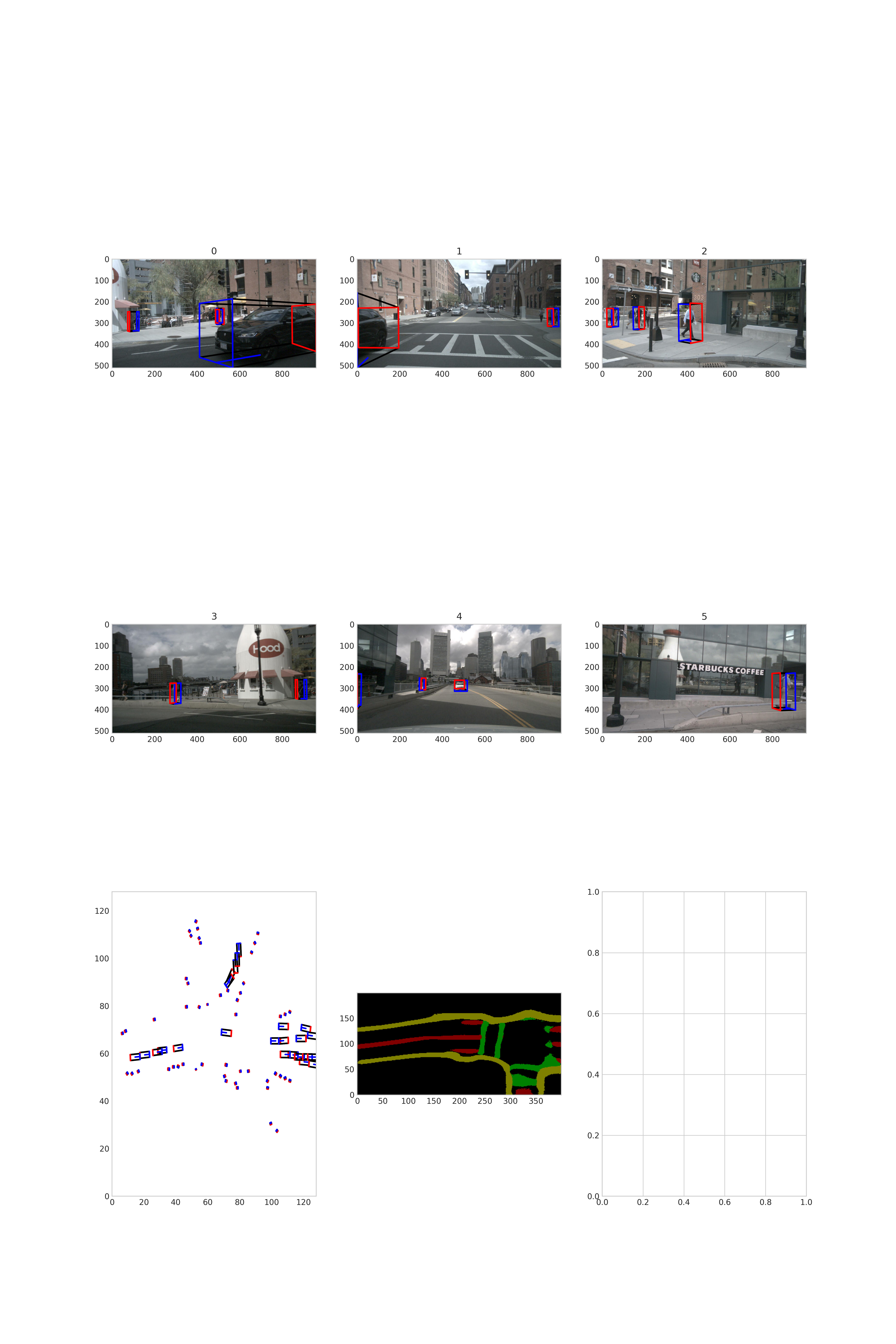
5.1 结果可视化-
如果你希望可以看到训练出来的模型对于单帧的检测效果,我们的tools文件夹下面同样提供了单帧预测及可视化的脚本, 你只需要按照infer.py中的格式给出每张图片的大小以及单应矩阵, 然后运行以下脚本即可:
python3 tools/infer.py --config configs/bev/bev_ipm_efficientnetb0_multitask_nuscenes.py --save-path ./
需在config文件中配置infer_cfg字段。
可视化结果将会在save-path路径下输出。
可视化示例:
6 板端部署-
6.1 上板性能实测-
使用hrt_model_exec perf工具将生成的.hbm文件上板做BPU性能FPS实测,hrt_model_exec perf参数如下:
hrt_model_exec perf --model_file {model}.hbm \
                    --thread_num 8 \
                    --frame_count 2000 \
                    --core_id 0 \
                    --profile_path '.'
6.2 AIBenchmark 示例-
OE开发包中提供了bev_ipm 的AI Benchmark示例,位于:ddk/samples/ai_benchmark/j5/qat/script/bev/bev_mt_ipm,具体使用可以参考开发者社区J5算法工具链产品手册-AIBenchmark评测示例-
可在板端使用以下命令执行做模型评测:
#性能数据
sh fps.sh
#单帧延迟数据
sh latency.sh
运行后会在终端打印出fps和latency数据。如果要进行精度评测,请参考开发者社区J5算法工具链产品手册-AIBenchmark示例精度评测 进行数据的准备和模型的推理。


