1 前言
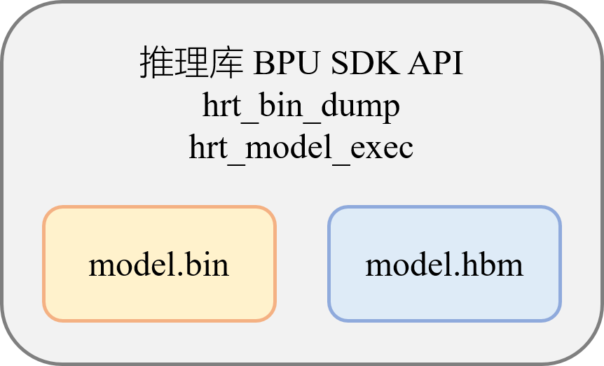
在完成模型的转换编译后,会得到可以在开发板上部署的模型文件,以bin或者hbm作为后缀名,区别在于:bin(Binary)模型是混合异构模型,可以同时包含CPU算子和BPU算子,而hbm(Horizon BPU Model)只含有BPU算子。这两种模型的板端部署方式没有区别,可以使用相同的推理库 BPU SDK API,也都支持hrt_bin_dump和hrt_model_exec工具对其进行分析。
2 示例介绍
OE包的ddk/samples/ai_toolchain/horizon_runtime_sample目录包含了板端部署的大量基础示例,code包含源码及编译相关文件,scrpit包含运行脚本及编译生成的可执行文件,预置了数据和相关模型,在开发板上运行script目录的脚本就可以执行对应的模型推理示例。-
本文重点介绍的快速上手示例是00_quick_start,这个示例会运行mobilenetv1_224x224_nv12.bin分类模型,读取一张jpg图片进行一次前向推理,并在后处理中计算得到Top5的分类结果。
开发者在编写板端部署代码前,需要先熟悉地平线提供的板端部署API,这部分可以查看工具链手册的BPU SDK API章节,这个章节除了详细介绍API接口,还全面介绍了板端部署有关的数据类型、数据接口等信息,以及数据排布与对齐规则,错误码等等。您也可以一边阅读示例代码,一边翻看API手册进行学习。
3 程序结构
-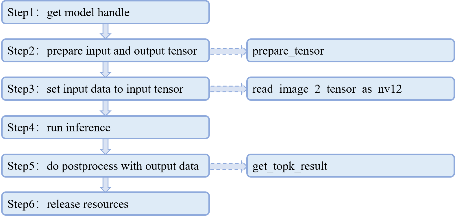
这张图展示了代码中main函数的六个主要步骤,实线箭头表示main函数的运行步骤,虚线箭头表示那个步骤需要调用的自定义函数,函数的具体实现在main函数之外。
4 代码解读
快速上手代码在OE开发包的路径为:-
ddk/samples/ai_toolchain/horizon_runtime_sample/code/00_quick_start/src/run_mobileNetV1_224x224.cc
DEFINE_string(model_file, EMPTY, "model file path");
DEFINE_string(image_file, EMPTY, "Test image path");
DEFINE_int32(top_k, 5, "Top k classes, 5 by default");
这里定义的字符串,代表板端运行脚本run_mobilenetV1.sh的命令行参数定义,即需要解析的输入参数,包括模型文件、图片文件,以及分类结果TopK的参数设置。
#define HB_CHECK_SUCCESS(value, errmsg)                              \
  do {                                                               \
    /*value can be call of function*/                                \
    auto ret_code = value;                                           \
    if (ret_code != 0) {                                             \
      VLOG(EXAMPLE_SYSTEM) << errmsg << ", error code:" << ret_code; \
      return ret_code;                                               \
    }                                                                \
  } while (0);
HB_CHECK_SUCCESS用于判断函数是否成功执行,参数value处填写执行的具体函数,函数返回值为0代表成功执行,执行失败则会返回错误码并在终端打印显示,用户可根据错误码对照工具链手册的5.2.5《错误码》章节查看报错原因,也可以使用hbDNNGetErrorDesc接口打印错误原因。
typedef struct Classification {
  int id;
  float score;
  const char *class_name;

  Classification() : class_name(0), id(0), score(0.0) {}
  Classification(int id, float score, const char *class_name)
      : id(id), score(score), class_name(class_name) {}

  friend bool operator>(const Classification &lhs, const Classification &rhs) {
    return (lhs.score > rhs.score);
  }

  ~Classification() {}
} Classification;
Classificaton结构体主要定义了三个变量,分别是分类序号id,分类得分score,以及类别名class_name,会在后处理计算TopK的时候使用,友元函数重载的>运算符是为了配合TopK计算中优先级队列的优先级设置,后文分析TopK代码的时候会进行详细介绍。
接下来我们跳过函数声明,直接进入main函数。
// Parsing command line arguments
  gflags::SetUsageMessage(argv[0]);
  gflags::ParseCommandLineFlags(&argc, &argv, true);
  std::cout << gflags::GetArgv() << std::endl;

  // Init logging
  google::InitGoogleLogging("");
  google::SetStderrLogging(0);
  google::SetVLOGLevel("*", 3);
  FLAGS_colorlogtostderr = true;
  FLAGS_minloglevel = google::INFO;
  FLAGS_logtostderr = true;

  hbPackedDNNHandle_t packed_dnn_handle;
  hbDNNHandle_t dnn_handle;
  const char **model_name_list;
  auto modelFileName = FLAGS_model_file.c_str();
  int model_count = 0;
这段代码使用了gflags的接口,解析脚本读取的文件信息并赋值给特定的变量。
// Step1: get model handle
  {
    HB_CHECK_SUCCESS(
        hbDNNInitializeFromFiles(&packed_dnn_handle, &modelFileName, 1),
        "hbDNNInitializeFromFiles failed");
    HB_CHECK_SUCCESS(hbDNNGetModelNameList(
                         &model_name_list, &model_count, packed_dnn_handle),
                     "hbDNNGetModelNameList failed");
    HB_CHECK_SUCCESS(
        hbDNNGetModelHandle(&dnn_handle, packed_dnn_handle, model_name_list[0]),
        "hbDNNGetModelHandle failed");
  }
Step1使用了三个API:从文件中初始化模型,获取模型的名称和数量,以及获取模型句柄。其中涉及到了“pack”的概念,这里做一个解释:工具链支持使用hb_pack工具将多个转换后bin模型整合成一个文件(使用细节可以查看工具链手册4.1.1.9《其他模型工具》),如果hbDNNInitializeFromFiles接口解析的是没有打包的单个模型,那么packed_dnn_handle指向的就是那一个模型,如果该接口解析的是打包了之后的整合模型,那么packed_dnn_handle会指向打包的多个模型,model_name_list列表也会包含所有的模型,model_count为所有模型的总数。
std::vector<hbDNNTensor> input_tensors;
  std::vector<hbDNNTensor> output_tensors;
  int input_count = 0;
  int output_count = 0;
// Step2: prepare input and output tensor
  {
    HB_CHECK_SUCCESS(hbDNNGetInputCount(&input_count, dnn_handle),
                     "hbDNNGetInputCount failed");
    HB_CHECK_SUCCESS(hbDNNGetOutputCount(&output_count, dnn_handle),
                     "hbDNNGetInputCount failed");
    input_tensors.resize(input_count);
    output_tensors.resize(output_count);
    prepare_tensor(input_tensors.data(), output_tensors.data(), dnn_handle);
  }
input_tensors和output_tensors是用vector定义的输入张量和输出张量,vector的数据类型是地平线封装的hbDNNTensor。input_count和output_count用于获取模型有多少个输入输出节点。之后进入Step2,调用hbDNNGetInputCount和hbDNNGetOutputCount接口,获取模型的输入输出节点数量,初始化input_count和output_count,再将输入张量input_tensors和输出张量output_tensors设定成对应的长度,用prepare_tensor函数进行内存空间的分配。接下来重点分析prepare_tensor函数(节选input部分):
int prepare_tensor(hbDNNTensor *input_tensor,
                   hbDNNTensor *output_tensor,
                   hbDNNHandle_t dnn_handle) {
  int input_count = 0;
  int output_count = 0;
  hbDNNGetInputCount(&input_count, dnn_handle);
  hbDNNGetOutputCount(&output_count, dnn_handle);

  hbDNNTensor *input = input_tensor;
  for (int i = 0; i < input_count; i++) {
    HB_CHECK_SUCCESS(
        hbDNNGetInputTensorProperties(&input[i].properties, dnn_handle, i),
        "hbDNNGetInputTensorProperties failed");
    int input_memSize = input[i].properties.alignedByteSize;
    HB_CHECK_SUCCESS(hbSysAllocCachedMem(&input[i].sysMem[0], input_memSize),
                     "hbSysAllocCachedMem failed");
    input[i].properties.alignedShape = input[i].properties.validShape;
    const char *input_name;
    HB_CHECK_SUCCESS(hbDNNGetInputName(&input_name, dnn_handle, i),
                     "hbDNNGetInputName failed");
    VLOG(EXAMPLE_DEBUG) << "input[" << i << "] name is " << input_name;
  }
  //output
  ......
  return 0;
}
prepare_tensor的主要作用是为输入输出张量分配合适的内存空间。如果模型有多个输入输出,则每个输入输出都会分配一次内存空间。hbDNNGetInputTensorProperties和hbDNNGetOutputTensorProperties用于从模型中解析输入输出张量的属性,input_memSize和output_memSize表示某个输入输出张量的对齐后的字节大小。-
其中有一条语句:input[i].properties.alignedShape = input[i].properties.validShape; 用于让板端推理库自动对图像类型的输入数据做对齐(不包含featuremap类型)。关于为输入数据做对齐的具体方法,可以查看社区文章《在部署时为输入数据做padding》,具体的对齐规则解析可以查看《模型输入输出对齐规则解析》。模型的alignedShape和validShape可以在板端使用hrt_model_exec工具的model_info功能查看。-
之后,使用hbSysAllocCachedMem接口分配带有缓存(Cache)的内存空间,有了缓存,CPU的读写效率会比不带缓存高很多。分配完内存空间后会打印当前输入输出节点的具体名称。
// Step3: set input data to input tensor
  {
    HB_CHECK_SUCCESS(
        read_image_2_tensor_as_nv12(FLAGS_image_file, input_tensors.data()),
        "read_image_2_tensor_as_nv12 failed");
    VLOG(EXAMPLE_DEBUG) << "read image to tensor as nv12 success";
  }
接下来回到主函数的Step3,在为输入输出张量分配完内存空间后,需要使用read_image_2_tensor_as_nv12函数将图像数据存放到输入张量对应的内存空间中。这个示例是从本地文件中读取rgb图像并转换成nv12作为模型的输入,如果处理视频通路输入的图像,可以参考全流程示例,即OE包的ddk/samples/ai_forward_view_sample,详细介绍可以查看社区文章《J5全流程示例解读》。
int32_t read_image_2_tensor_as_nv12(std::string &image_file,
                                    hbDNNTensor *input_tensor) {
  hbDNNTensor *input = input_tensor;
  hbDNNTensorProperties Properties = input->properties;
  int tensor_id = 0;
  // NCHW , the struct of mobilenetv1_224x224 shape is NCHW
  int input_h = Properties.validShape.dimensionSize[2];
  int input_w = Properties.validShape.dimensionSize[3];

  cv::Mat bgr_mat = cv::imread(image_file, cv::IMREAD_COLOR);
  if (bgr_mat.empty()) {
    VLOG(EXAMPLE_SYSTEM) << "image file not exist!";
    return -1;
  }
  // resize
  cv::Mat mat;
  mat.create(input_h, input_w, bgr_mat.type());
  cv::resize(bgr_mat, mat, mat.size(), 0, 0);
  // convert to YUV420
  if (input_h % 2 || input_w % 2) {
    VLOG(EXAMPLE_SYSTEM) << "input img height and width must aligned by 2!";
    return -1;
  }
  cv::Mat yuv_mat;
  cv::cvtColor(mat, yuv_mat, cv::COLOR_BGR2YUV_I420);
  uint8_t *nv12_data = yuv_mat.ptr<uint8_t>();

  // copy y data
  auto data = input->sysMem[0].virAddr;
  int32_t y_size = input_h * input_w;
  memcpy(reinterpret_cast<uint8_t *>(data), nv12_data, y_size);

  // copy uv data
  int32_t uv_height = input_h / 2;
  int32_t uv_width = input_w / 2;
  uint8_t *nv12 = reinterpret_cast<uint8_t *>(data) + y_size;
  uint8_t *u_data = nv12_data + y_size;
  uint8_t *v_data = u_data + uv_height * uv_width;

  for (int32_t i = 0; i < uv_width * uv_height; i++) {
    if (u_data && v_data) {
      *nv12++ = *u_data++;
      *nv12++ = *v_data++;
    }
  }
  return 0;
}
read_image_2_tensor_as_nv12函数的输入参数中,image_file是输入图片,input_tensor是输入张量。用opencv的imread接口读取到的图片是bgr类型的数据,会先将其resize成模型需要的尺寸,并转换成yuv420(即nv12)格式,之后将yuv420的图片数据拷贝到输入张量的内存空间当中。
hbDNNTaskHandle_t task_handle = nullptr;
  hbDNNTensor *output = output_tensors.data();
  // Step4: run inference
  {
    // make sure memory data is flushed to DDR before inference
    for (int i = 0; i < input_count; i++) {
      hbSysFlushMem(&input_tensors[i].sysMem[0], HB_SYS_MEM_CACHE_CLEAN);
    }

    hbDNNInferCtrlParam infer_ctrl_param;
    HB_DNN_INITIALIZE_INFER_CTRL_PARAM(&infer_ctrl_param);
    HB_CHECK_SUCCESS(hbDNNInfer(&task_handle,
                                &output,
                                input_tensors.data(),
                                dnn_handle,
                                &infer_ctrl_param),
                     "hbDNNInfer failed");
    // wait task done
    HB_CHECK_SUCCESS(hbDNNWaitTaskDone(task_handle, 0),
                     "hbDNNWaitTaskDone failed");
  }
接下来是主函数的Step4,我们现在已经读取了模型,为输入输出张量分配了内存空间,并且将待推理的图像数据存放到了输入张量的内存空间中,马上就可以进行前向推理了。但是在正式调用hbDNNInfer接口执行推理前,还需要有一些准备工作,首先使用hbDNNTaskHandle_t接口创建一个新的推理任务,并将任务句柄task_handle初始化为空指针,再设置output指针指向输出张量。由于我们为输入张量分配的内存是带有缓存的,所以需要先将缓存数据更新到内存,确保BPU能读取正确的数据。初始化推理的控制参数之后,就可以使用hbDNNInfer接口执行前向推理了。task_handle是任务句柄,output是输出张量,input_tensors是输入张量,dnn_handle是模型句柄。infer_ctrl_param是推理任务的控制参数,可以设置当前任务运行在哪个BPU核上,也可以设置当前任务的优先级,可以使用HB_DNN_INITIALIZE_INFER_CTRL_PARAM进行默认的初始化设置,具体如下:
bpuCoreId = HB_BPU_CORE_ANY;-
dspCoreId = HB_DSP_CORE_ANY;-
priority = HB_DNN_PRIORITY_LOWEST;-
customId = 0;-
reserved1 = 0;-
reserved2 = 0;
最后,hbDNNWaitTaskDone接口用于等待推理任务完成。
// Step5: do postprocess with output data
  std::vector<Classification> top_k_cls;
  {
    // make sure CPU read data from DDR before using output tensor data
    for (int i = 0; i < output_count; i++) {
      hbSysFlushMem(&output_tensors[i].sysMem[0], HB_SYS_MEM_CACHE_INVALIDATE);
    }

    get_topk_result(output, top_k_cls, FLAGS_top_k);
    for (int i = 0; i < FLAGS_top_k; i++) {
      VLOG(EXAMPLE_REPORT) << "TOP " << i << " result id: " << top_k_cls[i].id;
    }
  }
Step5是后处理的TopK计算。首先会定义一个名为top_k_cls的vector数组,这个数组的属性是Classification,也就是之前定义过的结构体,里面含有类的序号,分类得分,还有类的名字,这个vector数组用于存放TopK数量的信息,最后通过VLOG来打印结果。在执行TopK计算前,还需要将BPU输出数据从内存同步到缓存里,这样才能让CPU取到正确的数值。
void get_topk_result(hbDNNTensor *tensor,
                     std::vector<Classification> &top_k_cls,
                     int top_k) {
  hbSysFlushMem(&(tensor->sysMem[0]), HB_SYS_MEM_CACHE_INVALIDATE);
  std::priority_queue<Classification,
                      std::vector<Classification>,
                      std::greater<Classification>>
      queue;
  int *shape = tensor->properties.validShape.dimensionSize;
  // The type reinterpret_cast should be determined according to the output type
  // For example: HB_DNN_TENSOR_TYPE_F32 is float
  auto data = reinterpret_cast<float *>(tensor->sysMem[0].virAddr);
  auto shift = tensor->properties.shift.shiftData;
  auto scale = tensor->properties.scale.scaleData;
  int tensor_len = shape[0] * shape[1] * shape[2] * shape[3];
  for (auto i = 0; i < tensor_len; i++) {
    float score = 0.0;
    if (tensor->properties.quantiType == SHIFT) {
      score = data[i] / (1 << shift[i]);
    } else if (tensor->properties.quantiType == SCALE) {
      score = data[i] * scale[i];
    } else {
      score = data[i];
    }
    queue.push(Classification(i, score, ""));
    if (queue.size() > top_k) {
      queue.pop();
    }
  }
  while (!queue.empty()) {
    top_k_cls.emplace_back(queue.top());
    queue.pop();
  }
  std::reverse(top_k_cls.begin(), top_k_cls.end());
}
我们仔细分析一下get_topk_result这个函数:
-
函数有三个输入,tensor是输出的张量,top_k_cls是刚才定义了的vector数组,top_k指top_k个最高的得分,在这个示例中top_k是5。
-
在这个函数的具体实现中,首先定义了一个优先级队列queue,这个优先级队列的元素比较方式是greater,意思是数值越小优先级越高。在使用这个queue之前,会先判断这个模型的输出数据是否需要做反量化,如果需要做反量化,还会判断是shift类型还是scale类型。
-
浮点数据score表示的就是某一个类别最后的得分。每得到一个score,就会将这个score对应的类别送入优先级队列queue,如果queue的元素数量超过top_k,到达了6个,就会让queue中优先级最高的类别出队,又因为这个优先级队列数值最小的类优先级最高,所以出队的一定是这6个类中得分最低的类。这样循环完一整轮之后,优先级队列queue就只会剩下5个得分最高的类了。
-
最后再把queue里的数据存放到vector数组top_k_cls中进行打印,完成整个TopK的后处理逻辑。
// Step6: release resources
{
// release task handle
HB_CHECK_SUCCESS(hbDNNReleaseTask(task_handle), “hbDNNReleaseTask failed”);
// free input mem
for (int i = 0; i < input_count; i++) {
HB_CHECK_SUCCESS(hbSysFreeMem(&(input_tensors[i].sysMem[0])),
“hbSysFreeMem failed”);
}
// free output mem
for (int i = 0; i < output_count; i++) {
HB_CHECK_SUCCESS(hbSysFreeMem(&(output_tensors[i].sysMem[0])),
“hbSysFreeMem failed”);
}
// release model
HB_CHECK_SUCCESS(hbDNNRelease(packed_dnn_handle), “hbDNNRelease failed”);
}
主函数中的最后一步Step6,就是一些收尾工作,依次释放任务句柄,释放输入输出申请的内存空间,最后释放模型句柄。到这里,整个快速上手的代码就解读完成了。
5 板端运行
00_quick_start这个示例有两种运行方式,第一种是在x86端使用模拟器运行,第二种是在板端实际运行,接下来以j5芯片为例进行介绍,xj3的步骤类似。
- x86端模拟运行的方法是:先运行code文件夹下的build_x86.sh脚本,脚本执行完毕后会在j5文件夹下生成可执行文件及相关依赖,之后我们进入j5/script_x86/00_quick_start目录,运行run_mobilenetV1.sh脚本,即可以x86模拟器的方式运行该示例,执行模型的前向推理并打印Top5分类结果。
- 板端运行的具体方法是:先运行code文件夹下的build_j5.sh脚本,脚本执行完毕后会在j5文件夹下生成文件及相关依赖,我们将整个j5文件夹复制到板端,再进入j5/script/00_quick_start目录,运行run_mobilenetV1.sh脚本,即可在开发板上运行快速上手示例了。
这个快速上手示例在J5开发板上运行的终端打印信息如下:
I0000 00:00:00.000000 10765 vlog_is_on.cc:197] RAW: Set VLOG level for "*" to 3[BPU_PLAT]BPU Platform Version(1.3.3)!
[HBRT] set log level as 0. version = 3.15.18.0
[DNN] Runtime version = 1.17.2_(3.15.18 HBRT)[A][DNN][packed_model.cpp:225][Model](2023-04-11,17:51:17.206.804) [HorizonRT] The model builder version = 1.15.0
I0411 17:51:17.244180 10765 run_mobileNetV1_224x224.cc:135] DNN runtime version: 1.17.2_(3.15.18 HBRT)
I0411 17:51:17.244376 10765 run_mobileNetV1_224x224.cc:252] input[0] name is data
I0411 17:51:17.244508 10765 run_mobileNetV1_224x224.cc:268] output[0] name is prob
I0411 17:51:17.260176 10765 run_mobileNetV1_224x224.cc:159] read image to tensor as nv12 success
I0411 17:51:17.262075 10765 run_mobileNetV1_224x224.cc:194] TOP 0 result id: 340
I0411 17:51:17.262118 10765 run_mobileNetV1_224x224.cc:194] TOP 1 result id: 292
I0411 17:51:17.262148 10765 run_mobileNetV1_224x224.cc:194] TOP 2 result id: 282
I0411 17:51:17.262177 10765 run_mobileNetV1_224x224.cc:194] TOP 3 result id: 83
I0411 17:51:17.262205 10765 run_mobileNetV1_224x224.cc:194] TOP 4 result id: 290
可以看到,程序成功调用模型执行了一帧推理,并打印了Top5分类结果。-
希望本文能帮您快速上手模型的板端推理。